Genetic Diversity and Management Implications For Vicuña Populations In Peru

J.C. Wheeler¹, M. Fernandez², R. Rosadio², D.. Hoces³, M. Kadwell⁴, M.W.
Buford⁵

¹ CONOPA, Los Cerezos 106, Lima 3, Perú; email jwheeler@conopa.org;
² Facultad de Medicina Veterinaria, Universidad San Marcos, Lima, Perú;
³ Consejo Nacional de Camelidos Sudamericanos, CONACS, Lima, Perú;
⁴ Conservation Genetics Group, Institute ofo Zoology, Regent's Park, London, U.K.;
⁵ Cardiff School of Biosciences, Cardiff University, Cardiff, U.K.

1. INTRODUCTION

The scientific aims of this Darwin Initiative-funded project were to use molecular genetic markers (specifically microsatellites) to:

(1) elucidate the recent evolutionary history of Peruvian vicuña populations; (2) evaluate the genetic diversity and its partitioning in those populations; (3) identify demographically independent management units within these populations for future management; and (4)assess the likely genetic effects of past and future management strategies, including the likely consequences of sustainable utilisation practices. It is important to emphasise that this is the first such study carried out on a wild South American camelid.

2. SAMPLING RATIONALE AND STRATEGY

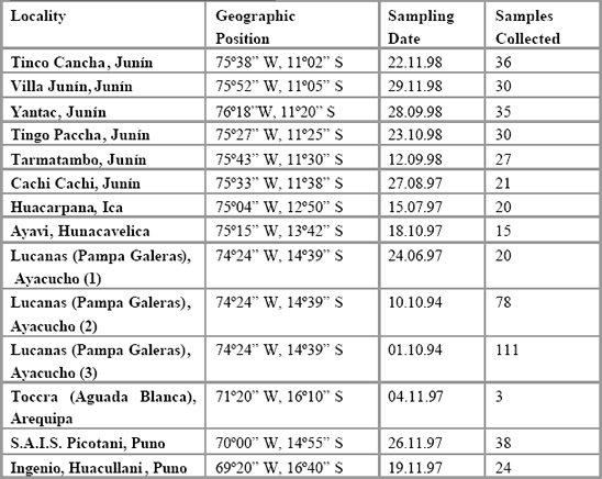
A total of 12 populations were sampled at sites selected for the following reasons: (1)geographic locations throughout the range of habitat and reserve coverage in Peru; (2)because they were thought to have had relatively long histories of demographic isolation; and (3)because they were thought not to have been influenced by recent translocations of animals from the Pampa Galeras reserve.

Table 1 details the geographic location of each sample, sample size, type and further details. Half of each sample was deposited in the Unidad de Virología y Genética Molecular laboratory at IVITA, and the remainder was sent to the Institute of Zoology for analysis, under Peruvian CITES export permits 00240 and 00658, and UK/EU CITES import permits 67264 and 206242/01. Samples used in this study were either blood or skins. 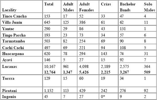Table 2 details what is known from the 1997 and 1999 CONACS census regarding demographic composition of each population. An indication of any anecdotal evidence of recent demographic fluctuation is also given.

Table 1. Vicuña sample location details

Notes: all samples were blood except for Ayacucho (3)which were skin taken from hides of
animals culled between 1977–1983.

Table 2. Demographic structure of Peruvian Vicuña populations. (Data from CONACS 1997 and 1999 censuses).

Notes: (1)crías are both sexes; (2)all populations stable, except for Ayavi (hunted), Lucanas
(recovering from less than 1000 individuals in 1963–64), Toccra (recovering); (3)Ingenio data
from February census; (4) 1999 census data in bold.

3. METHODS

Once the samples had been collected, DNA was extracted from blood or skin using standard procedures involving Proteinase K digestion of cellular material followed by nucleic acid extraction using phenol and phenol/chloroform to remove proteins, and total DNA was precipitated in 100 percent ethanol (see Bruford et al. 1998). DNA samples were stored suspended in TE solution (10 mM Tris–HCl, 1 mM EDTA, pH 8.0) prior to analysis.

Eleven previously published South American camelid (SAC) microsatellite DNA markers were analysed (Lang et al. 1996, Penedo et al. 1998). Microsatellites are nuclear (n)DNA markers found in the chromosomes of most eukaryotes and have been found to be highly polymorphic in many species, leading to their use in applications such as paternity testing, individual profiling in forensics, population analysis and hybridisation studies (Goldstein and Schlötterer 1999). We have previously shown that microsatellites can be used effectively in hybridisation studies involving SACs (Kadwell et al. 2001) and for the purposes of this study we used these markers to measure population genetic diversity and infer recent demographic history. Table 3 shows details of the microsatellites used, their genetic diversity in terms of heterozygosity (the proportion of individuals who inherit different alleles at a given gene or locus from their parents– a robust indicator of genetic variation) and allele sizes in Peruvian vicuña.

Table 3. Summary of genetic markers.

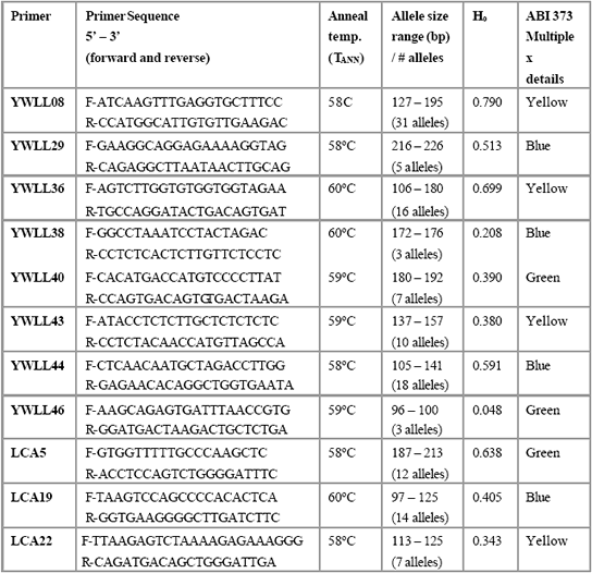
*Notes : (1)H0 mean observations heterozygosity ; (2)data source : YWLL08–YWLL46, Lang
et al. (1996) ; LCA5–LCA22, Penedo et al. (1998).

Table 4 breaks down this analysis of genetic diversity into data for each population and compares observed heterozygosity, expected heterozygosity (assuming breeding which is random with respect to the genetic similarity of the individuals) and mean number of alleles per locus. A large difference between observed and expected heterozygosity can be caused by non– random mating (e.g., inbreeding) or selection acting against certain genotypes.

Table 4. Genetic diversity in vicuña populations of Peru.

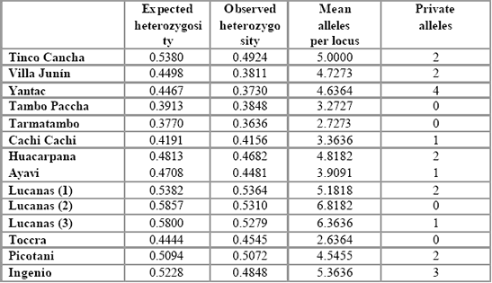
Table 5 indicates pair–wise values of genetic differentiation between populations measured by the commonly-used index F_ST, which varies between zero (no genetic differentiation) and one (complete differentiation) and can also be regarded as the component of the total genetic variation in any two populations which is attributable to the differences between them. F_ST is simply calculated as:

F_ST = H_T – H_S/ H_T,

where H_T is the expected heterozygosity in the total population and H_S is the expected heterozygosity in the sub-population in question. Table 5 also includes values of Nm, the estimated number of migrants per generation, which is calculated from F_ST using the formula:

Nm = (1–F_ST)/4F_ST,

which is included primarily for illustration, since this calculation makes assumptions about the populations that are certainly violated in some cases. All calculations and analytical approaches were implemented using the programs GENEPOP v3.1(Raymond and Rousset 1995) and GENETIX v4.0 (Belkhir 1999).

Table 5. Pairwise F_ST values (above diagonal) and Nm values (below diagonal) between populations in Peru.

Table 5 (continued). Pairwise F_ST values (above diagonal) and Nm values (below diagonal) between populations in Peru.

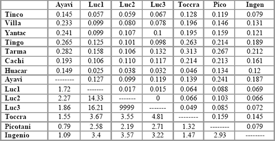
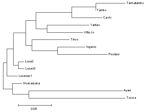
Figure 1 shows a dendrogram (genealogical tree of populations) generated using neighbour–joining analysis (Saitou et al. 1985) in the computer program MEGA (Kumar et al. 1993), which clusters populations according to their Nei’s 1972 genetic distance (Nei 1987, which analyses genetic variation in a way analogous to FST) and enables clusters of related populations to be identified. Figures 3a–d show 2–dimensional factorial correspondence plots of four populations in northwest Junín, south Junín, central Andes (Huancavelica–Arequipa) and Puno, respectively, where the genetic diversity among populations is expressed as factors which explain the correspondence among samples in a number of dimensions (here we show the two dimensions which explain the highest proportion of the correspondence according to Benzécri 1973; using GENETIX v. 4.0– see results for a fuller exp lanation). Thus the spatial relationships (approximate locations) between populations can be adjudged by examining how individuals from each population cluster in 2, 3 or more dimensions.

Figure 1. Neighbour–joining tree of Nei’s (1972) genetic distances between Peruvian vicuña populations.

Figure 2a. Northwest Junín (Yantac in black)

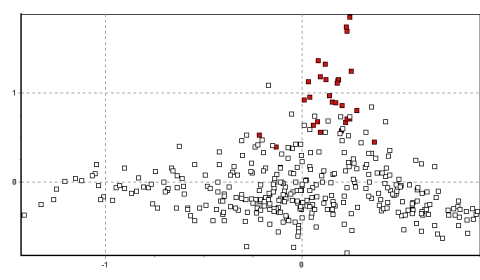
Figure 2b. South Junín (Tambo Paccha in black)

Figure 2c. Central Andes (Lucanas 2 in black)

Figure 2d. Puno (Picotani in black)

4. RESULTS AND INFERENCE

4.1 Population and Genetic Variation

4.1.1 Microsatellites

Table 3 shows that the markers used are highly polymorphic and informative in Peruvian vicuña, which means that they are ideal for study genetic diversity and differentiation. For example, YWLL08 is exceptionally informative and possesses 31 alleles and nearly 80 percent of individuals are heterozygotes. Interestingly, we have found many alleles previously unrecorded by the researchers who first developed them. For example, Lang et al. (1996), who isolated the YWLL markers used in this study from llama DNA, identified 13 alleles at YWLL 08 and 6 alleles at YWLL 36 (as opposed to 31 and 16 respectively in this study). Likewise, Penedo et al. (1998), who isolated the LCA microsatellites used here from llama DNA, found 7 alleles at LCA 5 and 10 alleles at LCA 22 (as opposed to 12 and 14 respectively in this study). However, the overall levels of heterozygosity are very much lower in this study compared with the original papers.

This is perhaps surprising, given that we have sampled wild populations of vicuña and compared them to domestic camelids. This result is most likely to be due to Peruvian vicuñas having lower genetic variation within populations, although this would seem counter–intuitive, given that vicuña possess so many more alleles than their domestic counterparts. This may be explicable, however, if that majority of genetic diversity in Peruvian vicuña is found between as opposed to within populations.

An alternative explanation is the phenomenon known as “ascertainment bias” where because we have used llama –derived microsatellites (which have been chosen to be highly polymorphic in llamas) in vicuña, they are more likely to be less variable precisely because they have not been chosen because of their diversity in vicuña. Furthermore, our previous data (Kadwell et al. 2001) indicate that llamas are the domestic camelid derived from guanacos. It is a commonly observed phenomenon that microsatellites isolated in a given species (here llama) are less variable in other species, regardless of how closely related they are. However, until such a time as an equivalent guanaco data set becomes available it is difficult to assess the relative contributions of the two potential explanatory factors, and it is possib le (indeed, likely) that both may be involved.

4.1.2 Populations –Genetic Diversity

Table 4 shows the levels of heterozygosity found in all populations analysed. Mean expected heterozygosity values over all loci vary between 0.377 (Tarmatambo) and 0.586 (Lucanas 2). These values are certainly lower than those commonly found in continental mammal populations (data not shown) which usually do not fall below 0.5 and thereby may reflect a recent history of population isolation with correlated genetic drift or may be a consequence of the type of microsatellites being used (see above). However, since the phenomenon seems to be found in many of the loci used, genetic drift or inbreeding may be likely.

This hypothesis is supported by the observations shown in Table 4, wherein observed heterozygosity is lower than expected heterozygosity (i.e., the value expected from the observed
allelic frequencies under the assumption of random mating) in all populations except one (Toccra, which suffers from a small sample size and may be biased). Such an observation is consistent with localised inbreeding or selection against heterozygotes. Furthermore, there is a significant excess
of homozygosity in all populations except Huacarpana, Lucanas 1, Cachi Cachi, Toccra and Tarmatambo (GENEPOP analysis), which suggests that inbreeding and/or genetic drift is a fairly common occurrence.

Inbreeding results from mating between relatives, and can be measured by an inbreeding coefficient, F, which varies between 0 and 1, but where values above 0.05 are considered high. For example, brother/sister mating results in an F–value of 0.25. Inbreeding in vicuña, however, is highly unlikely under normal circumstances because of the social system, where both sexes disperse from their natal group. A generally elevated inbreeding coefficient can, however, follow from a situation where a population has been through a major crash or demographic “bottleneck.”.

Table 4 also shows a total of 20 private (population–specific) alleles which is also higher than expected for a continental population sample and is further suggestive of some level of local isolation and genetic drift.

Interestingly the frequency of private alleles does not appear to correspond with population size or degree of isolation, although the northernmost population (Yantac) does possess the highest number of unique alleles. Finally, although it is clear that the allelic diversity of the entire population is high in comparison to the domestic populations chosen by Lang et al. (1996) and Penedo et al. (1998), the mean number of alleles per locus within populations is lower than often observed in other mammals (e.g., Tarmatambo with 2.7 alleles/locus), and it is only the Lucanas 2 and 3 that show the relatively high allelic diversity often associated with such studies.

4.1.3 Populations –Genetic Differentiation

Pairwise indices of genetic differentiation between populations (FST, Nei’s 1972 D) were measured and used to infer relationships between populations, calculate migration rates between them, and in combination with clustering methods, were used to graphically display inferred demographic clusters between them. Table 5 shows pairwise FST values between all populations, and the values vary between 0 in the case of Lucanas 2 and Lucanas 3 indicating complete genetic similarity (in this case not surprising since the samples were taken from the same population) and 0.31 between Toccra and Tarmatambo, a high degree of genetic differentiation between two continental mammal populations. In general, FST values are high, with 67 percent exceeding 0.1, all comparisons except two being significant at the p < 0.05 level and all except eight being significant p< 0.01. However, the values broadly reflect the known demographic relationships among the populations, with the lowest values being recorded between the Lucanas samples, and low values being found between populations in Puno and in south Junín.

Such population groups are clearly demographically dependent according to these data. Demographic dependence or independence can also be inferred from the Nm values shown below the diagonal in Table 5. Due to the generally high levels of FST found in the data set, many values of Nm are close to unity. An Nm value of one indicates that approximately one migrant is exchanged between two populations of equal size per generation (every n years), which
according to seminal work of Franklin and Soulé (1980) is sufficient to prevent divergence through genetic drift. The "one migrant per generation" (or OMPG) threshold has subsequently been used as a "rule of thumb" in management of populations to maintain demographic interdependence.

However, since the study populations vary in size considerably and because many are known to have been demographically isolated for hundreds of generations, such values are meaningless without being put into the context of known population history. For instance, it is surprising biogeographically that Yantac has supposedly exchanged 2.27 migrants per generation with
Lucanas 1 whereas it has only exchanged 1.12 with Cachi Cachi. Such results may partly be due to the biases mentioned above, and must be interpreted in the context of known population history. In general, the Nm values reflect apparent demographic history in the same way as the FST values, although some anomalous values appear which will be discussed later.

Genetic distances were also calculated, since they are thought to reflect the evolutionary history of populations more accurately than demographic indices such as FST (Nei 1987) and can be more effectively used by clustering algorithms such as neighbour–joining to produce dendrograms
which may reflect the evolutionary relationships between the populations being analysed. Here we used pair–wise Nei’s 1972 unbiased genetic distances (values not shown, although they broadly correlate with FST) to produce the neighbour–joining dendrogram shown in Figure 2 below.
Branch lengths are proportional to the genetic distance but do not imply evolutionary time scale since genetic distance values can be strongly influenced by demographic fluctuations too. However, generally the results enable us to infer relationships between populations that make both
biogeographical and demographic sense. For example, the three south Junín samples cluster closely together, as do two of the three northwest Junín samples and the two Puno samples. Less structure is apparent for the Lucanas, Huancavelica and Arequipa samples, however, which may be
indicative of a loose demographic affiliation between those populations not apparent in the genetic distance analysis.

Tinco Cancha is aberrant for reasons discussed below. Finally, the data were subjected to 2–dimensional factorial correspondence analysis (2D–FCA) to further explore the relationships
among populations. FCA is a canonical analysis particularly well adapted to describing relationships between two qualitative variables (here zero, one or two for each allele at each locus) which result in allele frequency vectors being produced for each population which are then analysed using Robertson and Hill’s FST estimator to produce a series of inertial values for each individual’s single locus FST estimates. Each axis of inertial values can be analysed in multidimensional space to produce a factorial correspondence plot, the most powerful of which represents the greatest proportion of the total inertial value. The result is a powerful method for recovering maximal
information on the genetic relationships among individuals within and between populations using n–dimensional space. For the vicuña data, the first two axes jointly explained approximately 6.5 percent of the total inertial value, a larger than average proportion for intraspecific analyses, and a reflection on the relatively high power of the data.

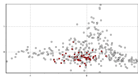
Figures 2a-d show the results for the entire data set in two dimensions. What is immediately apparent is the tight clustering of many of the individuals within each population and the unique locations which several of the populations occupy in 2–dimensional space. Of particular note are the populations of Picotani (Figure 2d: the only population found between vectors –0.6 and –1.2 on the ‘x’ axis), and Yantac (Figure 2a: the main population found between vectors 0.9 and 1.5 on the ‘y’ axis). In addition, several population groups become apparent due to their strong clustering in 2D space. Four broad groups are identifiable , and Figures 2a–d highlight
these and explain their origin. The populations of Yantac, Villa Junín and to a lesser extent Tinco Cancha in northwest Junín form a group occupying (x/y) 0–0.5/0.2–1.5 (see Fig 2a). Of these, Yantac, located at the northern extreme, is clearly the most different from the remainder of the population, with Villa Junín occupying 2D space intermediate with the south Junín samples. Tinco Cancha, however, has a more central distribution, similar to the Lucanas samples (see below and Fig 3).

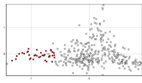
The populations in south Junín cluster tightly, occupying predominantly the (x/y) vector coordinate range of 0–0.5/–0.5–0: the bottom right hand section of the plot (see Figure 2b). This coordinate space is also unique among Peruvian vicuña populations, and strongly indicative of an
independent demographic history for this region.

A main feature of the 2D–FCA plots is a large cluster of populations in the centre of the vector distribution. This cluster comprises all the Lucanas samples, Ayavi, Huacarpana, Toccra and to a lesser extent Ingenio in Puno (x/y range –0.5 to 0.2/–0.8 to 0.5). These results recapitulate the genetic distance dendrograms in Figure 1 and suggest that the populations from Huancavelica, Ayacucho and Arequipa form a single demographically linked group of subpopulations, with some linkage to the Ingenio population south of Lake Titicaca in Puno. Of particular note is the strong relationship between the Huacarpana population and the samples from Lucanas (also evident from the FST data) and the fact that the Toccra data must be treated with caution because of the low sample size. Finally, the Puno population of Picotani seen in Figure 2d occupies its own 2D space (x/y = –1.5 to –0.5/–0.8 to 0.2) and is very distinctive.

Picotani is situated north of Lake Titicaca and not far from the Bolivian border. Its extreme distinctiveness (on a similar scale to Yantac) clearly requires particular attention.

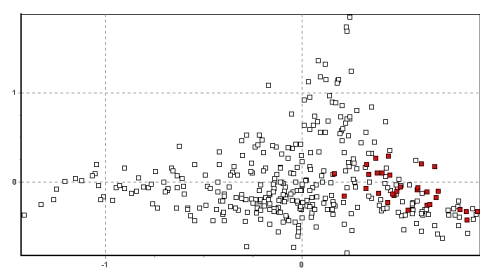
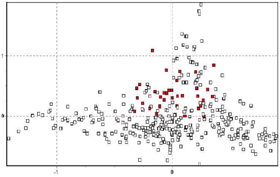
5. ANOMALOUS POPULATIONS

During the course of this study, clear patterns have emerged from the genetic data. However, several exceptions also emerged. First, the population in Tinco Cancha in north Junín genetically resembles the central Peruvian group much more than the northwestern Junín group (Figure 3),
with a similar effect evident to a lesser extent in Villa Junín. (In Figure 3, the points located between –0.3–0.2/0–0.5(x/y) correspond to descendants of animals transferred from Pampa Galeras, while those between –0.10– 0.4/0.1–1.1 (x/y) represent animals with the native northwest Junín group genotype.). Second, the sample from Huacarpana in Ica is genetically more
similar to the Lucanas populations than expected from its location.

It is now apparent that these populations have been affected by two large translocations from the Pampa Galeras reserve (Lucanas). These translocations have severely affected the genetic structure of the local Junín populations and future management strategies should take this into account. Other translocations from Pampa Galeras have occurred during the past 35 years. These include 722 vicuña to Laccho (Huancavelica) during 1979/1980; 40 vicuña to Caña guas (Parque Nacional Aguada Blanca– Arequipa) in 1979; 1012 vicuña to Atoxaico (Junín) in 1980/1981; 108 and 100 vicuña to Parque Nacional Huascarán–Ancash in 1980 and 1997, respectively; 25 and 170 vicuña to Cooperativa Atahualpa (Cajamarca) in 1994 and 1997, respectively; and 95 vicuña to Toccra (Parque Nacional Aguada Blanca–Arequipa) in 1997. Our study has documented the impact of the first and third in the genome of the local recipient populations, but the influence of transfers 2, 4 and 6 remains to be studied.

Figure 3. 2D-FCA plot with samples from Tinco Cancha, Junín in red.
The points located between -0.3-0.2/0-0.5(x/y) correspond to descendants of animals
transferred from Pampa Galeras, while those between -0.10-0.4/0.1-1.1 (x/y) represent
animals with the native northwest Junín group genotype.

6. CONCLUSIONS AND CONSERVATION

RECOMMENDATIONS

Vicuña populations in Peru seem to possess several interesting and strong genetic features, which are a result of its biology, habitat occupancy, evolutionary history and management by people in the recent past. First, the genetic diversity of Peruvian vicuña is characterised by relatively low levels of genetic diversity within populations, but high levels of genetic differentiation between populations. Such patterns are commonly observed in threatened species with formerly large ranges which have become isolated from each other and have suffered drastic demographic
contraction in recent generations (e.g., O’Ryan et al. 1998, Barratt et al. 1999). Such an effect may be predominating the genetic signal seen here in Peruvian vicuña, and should be acknowledged in future management strategies to minimise further loss of genetic diversity within individual vicuña populations.

It is especially important that future management strategies for fibre production in vicuña take account of the future genetic diversity of the populations and that the reproduction of individuals (especially males) be monitored and managed to maximise genetic diversity. Such an approach
includes provision for the free movement of individuals and precludes, for example, the exclusive use of a few productive males or of active selection programs to increase fibre productivity in wild populations, since they would be likely to lead to further inbreeding and genetic drift and thereby having deleterious effects on the health of individuals and overall wellbeing of the population. In addition, such an approach is unlikely to lead to an increase in fibre quality either, since domestication in other fibre producing species has universally led to a significant decrease in quality. Finally, it is important to note that the vicuña has already been domesticated and is undoubtedly the ancestor of the alpaca (Kadwell et al. 2001). However, the high numbers of private alleles and clear biogeographical structure of genetic diversity (see below) hints at an additional explanatory factor for the genetic patterns measured here. Andean animal populations are clearly occupying one of the most extreme and variable topographical environments in the world, and one where climate change, geological upheaval and changing colonisation routes must have a crucial role in shaping the genetic relationships among populations today.

It may be reasonable to expect many vicuña populations to have been naturally isolated, then perhaps reconnected, and then possibly isolated again throughout much of their history. These effects, coupled with the recent anthropogenic influence on vicuña populations, make it difficult to assess how much of the genetic pattern seen here is a result of recent human exploitation and how much is a natural consequence of evolutionary history.

A conservative approach to future management, however, would be to pay attention to the current patterns of genetic diversity described here, and to attempt to avoid future losses in diversity and structure. Second, we have identified four demographically distinct groups, those in northwest Junín, south Junín, central Andes (Huancavelica to Arequipa) and Puno. Such groups could conceivably form separate management units for future demographic augmentation within and between populations. Of particular note is the extreme northwestern population of Yantac, which is
genetically unique in this sample set and may represent a northern evolutionary group requiring special attention and further research. Also of note is the distinctiveness of the Puno population of Picotani, which conceivably represents a genetic group linked to the Bolivian population.

It is important, therefore, to establish the genetic relationships between the Picotani population and those in Bolivia and to assess both how far this genetic group penetrates into Peru and how much it differs from the south Puno Ingenio sample. The populations in southern Junín form a clearly independent demographic unit worthy of special consideration, and the large central Peruvian population, which includes the highly diverse population at Lucanas, appears to form a large demographic management unit. However, it should be noted that the Toccra sample analysed here is not large enough to form firm conclusions.

6.1 Recommendations

1. Vicuña populations in Peru should be conservatively managed in four demographic units (northwest Junín, except Tinco Cancha; south Junín; central Andes (Huancavelica to Arequipa); Puno).
2. Genetic management should be carried out by moving individuals between populations within the same management unit to prevent further loss of genetic diversity.
3. No further translocations should be carried out from Pampa Galeras to populations outside the Central Andes management unit because of the profound effect they may have on local genetic structure (for example in Tinco Cancha).
4. Genetic management within populations requires measures to minimise further inbreeding and genetic drift and this must be taken into account management practice for fibre production. Hence the free movement of individuals within localities must be ensured. If potential barriers to free
movement (e.g., fences) exist, large gaps should be kept open at all times, and these should only be closed for intensive management (i.e., chaccu).Further, since any fencing will act as a barrier to movement, methods of intensive management should be found which will lead to the elimination of fencing in the medium term.
5. Priority should be given to obtaining samples for genetic analysis from the region of Ancash, to see if populations comprise the same "northern" genotype as exemplified in Yantac.
6. Samples should be obtained to augment the current sample from Toccra (Aguada Blanca).
7. Samples should be obtained to further investigate the genetic status of the northern Puno group, both from Bolivia and from north and west of Picotani, to establish the penetration of this group into Peru.
8. Samples should be obtained from the area south of Lake Titicaca in Puno to further investigate how closely related these animals are to the north Puno and central Andes populations.
9. Phenotypic analysis (including of fibre) should be carried out on the four sub–populations identified here.
10. A simplified, short version of this report should be given wide circulation to interested parties, especially the campesinos.
11. A similar study should be carried out when possible on the guanaco populations in Perú.

7. ACKNOWLEDGEMENTS

We would like to acknow ledge the efforts of Dr. Helen F. Stanley at the Institute of Zoology for help with sampling and project design. We would also like to thank Valerie Richardson and Maria Stevens at the Darwin Initiative Secretariat, DETR London for much flexibility and help with
project management. At the Faculty of Veterinary Medicine, San Marcos University we would like to acknowledge the help of Dr. Felipe San Martin, Ing. Juan Olazabal and Antonina Cano. At CONACS we would like to thank Alfonso Martinez, Jorge Herrera, Marco Antonio Zuñiga, Marco Antonio
Escobar, Alex Montufar, Roberto Bombilla and all others who helped with the sampling. The research reported in this paper was carried out under Darwin Initiative for the Survival of Species grant 162/06/126.

8. REFERENCES

Barratt, E.M., Gurnell, J., Malarky, G., Deaville, R., and Bruford, M.W. 1999. Genetic Structure of fragmented populations of red squirrel (Sciurus vulgaris ) in Britain. Molecular Ecology S12: 55–65.

Belkhir, L. 1999. GENETIX v4.0. Belkhir Biosoft, Laboratoire des Genomes et Populations,
Université Montpellier II.

Benzécri, J.P. 1973. L’Analyse des Données: T. 2, I' Analyse des correspondances . Paris:
Dunod.

Bruford, M.W., Hanotte O., Brookfield J.F.Y., and Burke T. 1998. Single and multilocus DNA finge rprinting. In: Hoelzel, A.R. (Ed.) Molecular Genetic Analysis of Populations: A Practical Approach, 2nd Edition, Oxford University Press, Oxford.

Franklin, I., and Soulé, M. 1980 Conservation and Evolution. Longman, New York.

Goldstein, D., and Schlötterer, C. (Eds.). 1999. Microsatellites: Evolution and Applications.
Oxford University Press, Oxford.

Kadwell, M., Fernandez M., Stanley H.F., Baldi, R., Wheeler J.C., Rosadio R., and Bruford
M.W. 2001. Genetic analysis reveals the wild ancestors of the llama and alpaca.
Proceedings Royal Society of London B 268: 2575–1584.

Kumar, S., Tamura, K., and Nei, M. 1993. MEGA: Molecular Evolutionary Genetics Analysis, version 1.01. The Pennsylvania State University, University Park, PA 16802.

Lang, K.D.M., Wang Y., and Plante, Y. 1996. Fifteen polymorphic dinucleotide microsatellites in llamas and alpacas. Animal Genetics 27: 293.

Nei, M. 1987. Molecular Evolutionary Genetics. Columbia University Press, New York.

O’Ryan, C., Harley, E.H., Bruford, M.W., Beaumont, M.A., Wayne, R.K.Cherry, and M.I. 1998. Microsatellite analysis of genetic diversity in fragmented South African buffalo populations. Animal Conservation 1: 124–131.

Penedo M.C.T., Caetano A.R., and Cordova K.I. 1998. Microsatellite markers for South
American camelids. Animal Genetics 29: 411–412.

Raymond M., and Rousset F. 1995. GENEPOP (version 1.2): Population genetics software
for exact tests and ecumenicism. Journal of Heredity 86: 248–249

Saitou, N., and M. Nei. 1987. The neighbor joining method: A new method for reconstructing
phylogenetic trees. Molecular Biology and Evolution 4: 406–425.